Helen district heat generation dataset 2015-2020
I was notified yesterday that Helsinki district heating company Helen published their district heat generation data from 2015-2020. This is very nice indeed, since generation data has been notoriously hard to get as a researcher. I’m leaving here some notes on how to read the data in a Jupyter notebook.
See the announcement and link to dataset here, in Finnish.
In this post, we read in the Helen DH dataset and fix their timestamps. This content is also in Jupyter notebook format in GitHub
First, we request content from the server (link as of 2021-04-09) and inspect the data.
import requests
import pandas as pd

from io import StringIO

HELEN_DATA_URL = 'https://www.helen.fi/globalassets/helen-oy/vastuullisuus/hki_dh_2015_2020_a.csv'

content = requests.get(HELEN_DATA_URL).text
content[0:100]
'date_time;dh_MWh\r\n1.1.2015 1:00;936\r\n1.1.2015 2:00;924,2\r\n1.1.2015 3:00;926,3\r\n1.1.2015 4:00;942,1\r\n'
Fixing timestamps
It seems that there are two columns, first including a naive timestamp and second the generation in MWh per hour. Let’s read the data into a Pandas dataframe and then see to the timestamps
df = pd.read_csv(StringIO(content), sep=';', decimal=',', parse_dates=['date_time'], dayfirst=True)\
    .set_index('date_time')
df
| dh_MWh | |
|---|---|
| date_time | |
| 2015-01-01 01:00:00 | 936.000 |
| 2015-01-01 02:00:00 | 924.200 |
| 2015-01-01 03:00:00 | 926.300 |
| 2015-01-01 04:00:00 | 942.100 |
| 2015-01-01 05:00:00 | 957.100 |
| ... | ... |
| 2020-12-31 19:00:00 | 1191.663 |
| 2020-12-31 20:00:00 | 1155.601 |
| 2020-12-31 21:00:00 | 1149.378 |
| 2020-12-31 22:00:00 | 1097.287 |
| 2020-12-31 23:00:00 | 1110.583 |
52607 rows × 1 columns
Now, with naive timestamps there is most likely confusion with the daytime changes. Let’s two locations we know it happening, on 29th March 2015 03:00 and on 25th October 2020 at 4:00.
df.loc[((df.index >='2015-03-29 00:00') & (df.index < '2015-03-29 06:00'))
        | ((df.index >= '2020-10-25 00:00') & (df.index < '2020-10-25 06:00'))]
| dh_MWh | |
|---|---|
| date_time | |
| 2015-03-29 00:00:00 | 958.673 |
| 2015-03-29 01:00:00 | 930.965 |
| 2015-03-29 02:00:00 | 919.913 |
| 2015-03-29 04:00:00 | 913.885 |
| 2015-03-29 05:00:00 | 908.093 |
| 2020-10-25 00:00:00 | 871.322 |
| 2020-10-25 01:00:00 | 860.284 |
| 2020-10-25 02:00:00 | 848.808 |
| 2020-10-25 03:00:00 | 851.583 |
| 2020-10-25 03:00:00 | 842.317 |
| 2020-10-25 04:00:00 | 819.973 |
| 2020-10-25 05:00:00 | 820.491 |
So there it is, time hops two hours between 2015-03-29 02:00:00 and 2015-03-29 04:00:00,
and two similar timestamps exist at 2020-10-25 03:00:00. We will fix that next with tz_localize,
see documentation.
Ambiguous parameter ‘infer’ attempts to sort out autumn daylight saving time transition based on appearance order.
df.index = df.index.tz_localize(tz='Europe/Helsinki', ambiguous='infer')
df.loc[((df.index >='2015-03-29 00:00') & (df.index < '2015-03-29 06:00'))
        | ((df.index >= '2020-10-25 00:00') & (df.index < '2020-10-25 06:00'))]
| dh_MWh | |
|---|---|
| date_time | |
| 2015-03-29 00:00:00+02:00 | 958.673 |
| 2015-03-29 01:00:00+02:00 | 930.965 |
| 2015-03-29 02:00:00+02:00 | 919.913 |
| 2015-03-29 04:00:00+03:00 | 913.885 |
| 2015-03-29 05:00:00+03:00 | 908.093 |
| 2020-10-25 00:00:00+03:00 | 871.322 |
| 2020-10-25 01:00:00+03:00 | 860.284 |
| 2020-10-25 02:00:00+03:00 | 848.808 |
| 2020-10-25 03:00:00+03:00 | 851.583 |
| 2020-10-25 03:00:00+02:00 | 842.317 |
| 2020-10-25 04:00:00+02:00 | 819.973 |
| 2020-10-25 05:00:00+02:00 | 820.491 |
It seems correct now! Let’s check.
len(df.index.unique()) == len(df)
True
Finally, we will check that there is one hour difference between all rows
index_steps = df.index.to_frame().diff()
index_steps.loc[index_steps['date_time'] != pd.Timedelta('1 hours')]
| date_time | |
|---|---|
| date_time | |
| 2015-01-01 01:00:00+02:00 | NaT |
Basic plotting
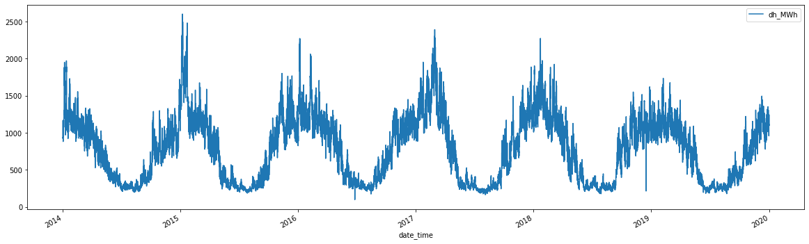
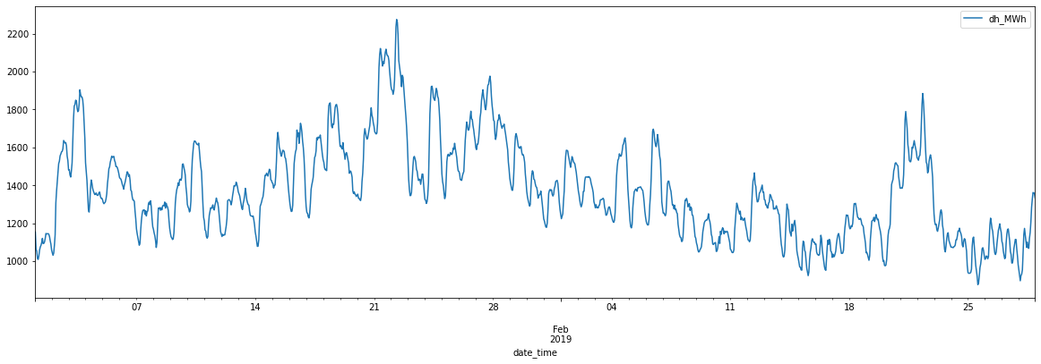
Let’s have a look at the data, plotted fully, and then a subplot
df.plot(figsize=(20,6))
<AxesSubplot:xlabel='date_time'>
df.loc[(df.index > '2019-01-01') & (df.index < '2019-03-01')].plot(figsize=(20,6))
<AxesSubplot:xlabel='date_time'>
Next steps
The data seems to be in order. Next one would like to plot correlations with the temperature, build models et cetera. This will be left for another time.